Mining in Wallapop
Hi! Today we’re going to do a bit of data science in Wallapop.
But what is Wallapop? A marketplace to buy or sell stuff that people no longer needs, usually within your area.
And what do we want? Mmmh… Let’s say we want to get a general view of what Spanish people are selling, who are the top sellers, how much are they making, what might be a star product, etc.
Data Analysis
Our goal is to goal discover useful information, suggesting conclusions, and supporting decision-making.
Data requirements
We need to collect at least two entities with at least some specific and key variables.
- Sellers:
ID,location,selling countandsold count. - Items:
ID,seller who sold it,category,name,sale price,published date,sold date.
Data collection
Our first option is to scrape their website, but as they seem to have an API Rest, let’s try to use it.
Building an API
On the website, URLs usually follow these patterns. They’re okay to get some IDs fast, but not ideal, so we have to find a way to get a *.json or similar in order to speed-up of data collection.
-
User ID:
https://es.wallapop.com/user/myfuturshop-75031299 User ID: 75031299 -
User photo:
https://cdn.wallapop.com/shnm-portlet/images?pictureId=429825383&pictureSize=W320 pictureId: 429825383 -
, etc.
API Rest
As they seem to use some kind of front-end web application framework, it would be convenient to capture the entire request and response (here I used Burp Suit to have more control over the requests).
- Choosing a region:
GET /maps/here/place?placeId=España, Comunitat Valenciana, València HTTP/1.1
Host: es.wallapop.com
User-Agent: Mozilla/5.0 (Macintosh; Intel Mac OS X 10.13; rv:59.0) Gecko/20100101 Firefox/59.0
Accept: application/json, text/javascript, */*; q=0.01
Accept-Language: en-US,en;q=0.8,es-ES;q=0.5,es;q=0.3
Accept-Encoding: gzip, deflate
Referer: https://es.wallapop.com/
X-Requested-With: XMLHttpRequest
Cookie: hideCookieMessage=true; session_id=03e9a435-99eb-4d1d-855e-3f9e245d8f85; userHasLogged=%7B%22hasLogged%22%3Afalse%2C%22times%22%3A1%7D; device_access_token_id=8047940e1707df337ad8dcff21a0598f; _ga=GA1.2.277003756.1525456570; _gid=GA1.2.180095070.1525456570; G_ENABLED_IDPS=google; __gads=ID=72f0aaff5a44463c:T=1525456575:S=ALNI_MZ0fp6uIwUf6Dnhs1UN98ncoGpZ4w
Connection: close
- Going to the next page:
GET /rest/items?kws=&_p=1&catIds=&searchNextPage=itemsCount%3D40%26start%3D40%26bumpCollectionType%3D0%26densityType%3D20%26step%3D0%26orderType%3Dasc%26keywords%3D%26latitude%3D39.46868%26orderBy%3Ddistance%26longitude%3D-0.37691 HTTP/1.1
Host: es.wallapop.com
User-Agent: Mozilla/5.0 (Macintosh; Intel Mac OS X 10.13; rv:59.0) Gecko/20100101 Firefox/59.0
Accept: */*
Accept-Language: en-US,en;q=0.8,es-ES;q=0.5,es;q=0.3
Accept-Encoding: gzip, deflate
Referer: https://es.wallapop.com/search?kws=&catIds=&verticalId=
X-Requested-With: XMLHttpRequest
Cookie: hideCookieMessage=true; session_id=03e9a435-99eb-4d1d-855e-3f9e245d8f85; userHasLogged=%7B%22hasLogged%22%3Afalse%2C%22times%22%3A1%7D; device_access_token_id=8047940e1707df337ad8dcff21a0598f; _ga=GA1.2.277003756.1525456570; _gid=GA1.2.180095070.1525456570; G_ENABLED_IDPS=google; __gads=ID=72f0aaff5a44463c:T=1525456575:S=ALNI_MZ0fp6uIwUf6Dnhs1UN98ncoGpZ4w; searchLat=39.46868; searchLng=-0.37691; searchPosName=Espa%C3%B1a%2C%20Comunitat%20Valenciana%2C%20Val%C3%A8ncia; bLat=39.4656217; bLng=-0.34386469999999997; _gat=1
Connection: close
Playing around with these, we can discover most filters:
_p: Page number (1)kws: Keywords, your query (iphone+8)catIds: Category IDs (12800, 14211,…)distanceSegments: Distance intervals ({min}_{max})dist: Maximum distance (400)salePriceSegments: Sale price intervals ({min.xx}_{max.xx})minPrice: Minimum price (15.00)maxPrice: Maximum price (200.00)markAsIds: shipping, exchange, urgentItemspublishDate: any, 30, 7, 24order: Ordering ({by}-{type}): creationDate-des, salePrice-des, salePrice-asc, distance-ascorderBy: creationDate, salePrice, salePriceorderType: des, asclatitude: 42.80785longitude: -2.30867
Using these parameters, we should be able to build URLs like this one:
https://es.wallapop.com/rest/items?_p=1&dist=400&publishDate=any&orderBy=distance&orderType=asc&latitude=42.80785&longitude=-2.30867
But then something happens… It’s doesn’t work as we expected. Why? Because we have to pass some parameters through the cookie values (at least the coordinates). Hence, our headers would be something like:
GET /rest/items?_p=24&dist=100&publishDate=any&orderBy=distance&orderType=asc&latitude=42.80785&longitude=-2.30867 HTTP/1.1

'Host': 'es.wallapop.com',
'User-Agent': 'Mozilla/5.0 (Macintosh; Intel Mac OS X 10.13; rv:59.0) Gecko/20100101 Firefox/59.0',
'Accept': 'text/html,application/xhtml+xml,application/xml;q=0.9,*/*;q=0.8',
'Accept-Language': 'en-US,en;q=0.8,es-ES;q=0.5,es;q=0.3',
'Accept-Encoding': 'gzip, deflate'
'cookie': 'searchLat=42.80785; searchLng=-2.30867;'
The above request should returned something like this:
APK decompiling
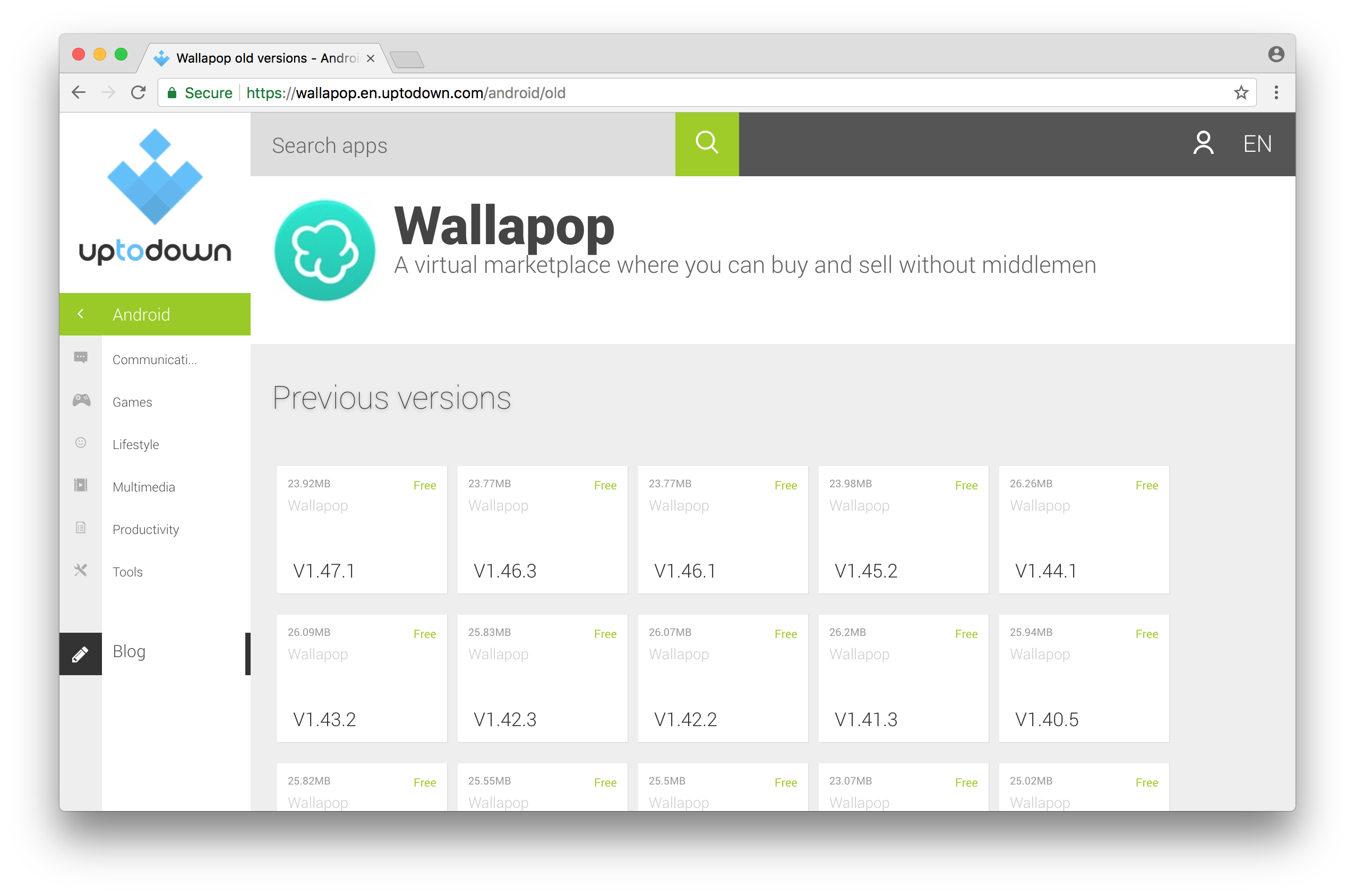
Okay, now we have an API but what if we could get more information? To do that, we’ll try to download a few versions of the Android app and decompile them.
In wallapop.en.uptodown.com we can find older versions of many apps, so just download a few.
Once, they’re downloaded we can decompile them using the following tools and look for files with the words: api, rest, latitude, urgentItems,… in it.
- Dex2jar: Tools to work with android .dex and java .class files
- ApkTool: A tool for reverse engineering Android apk files
- JD-GUI: Java Decompiler is a tool to decompile and analyze Java 5 “bytecode” and the later versions.
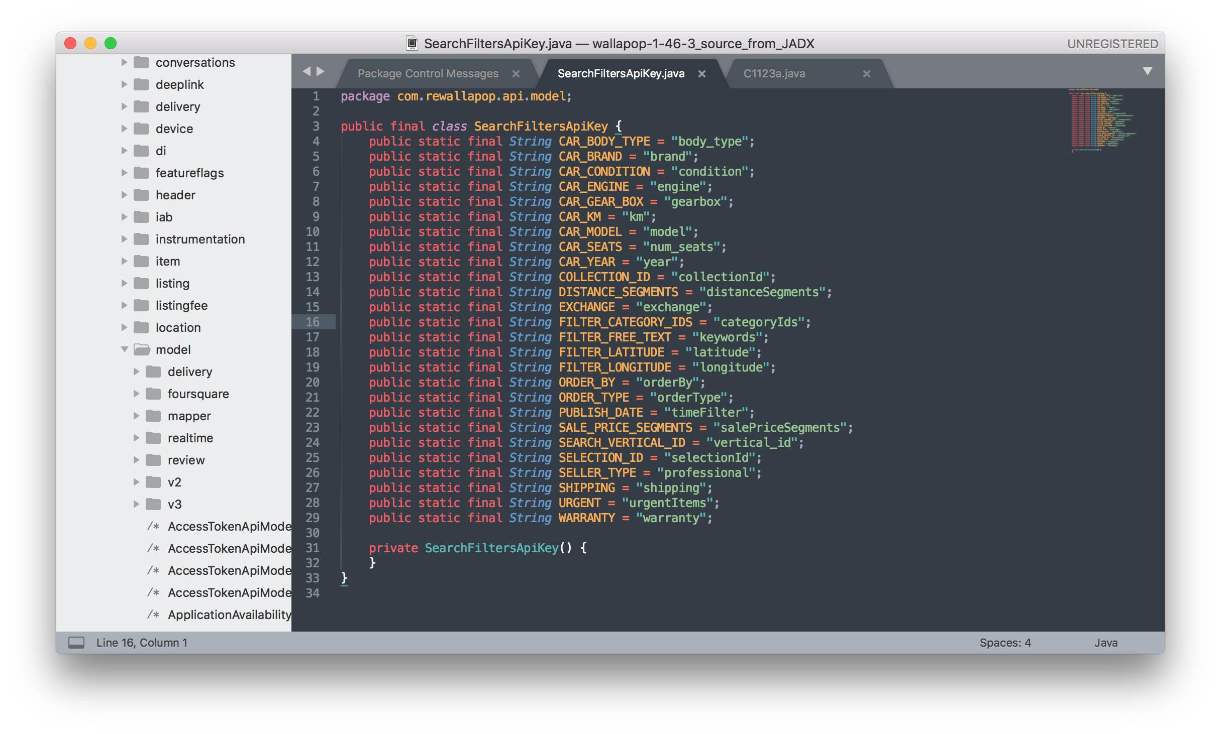
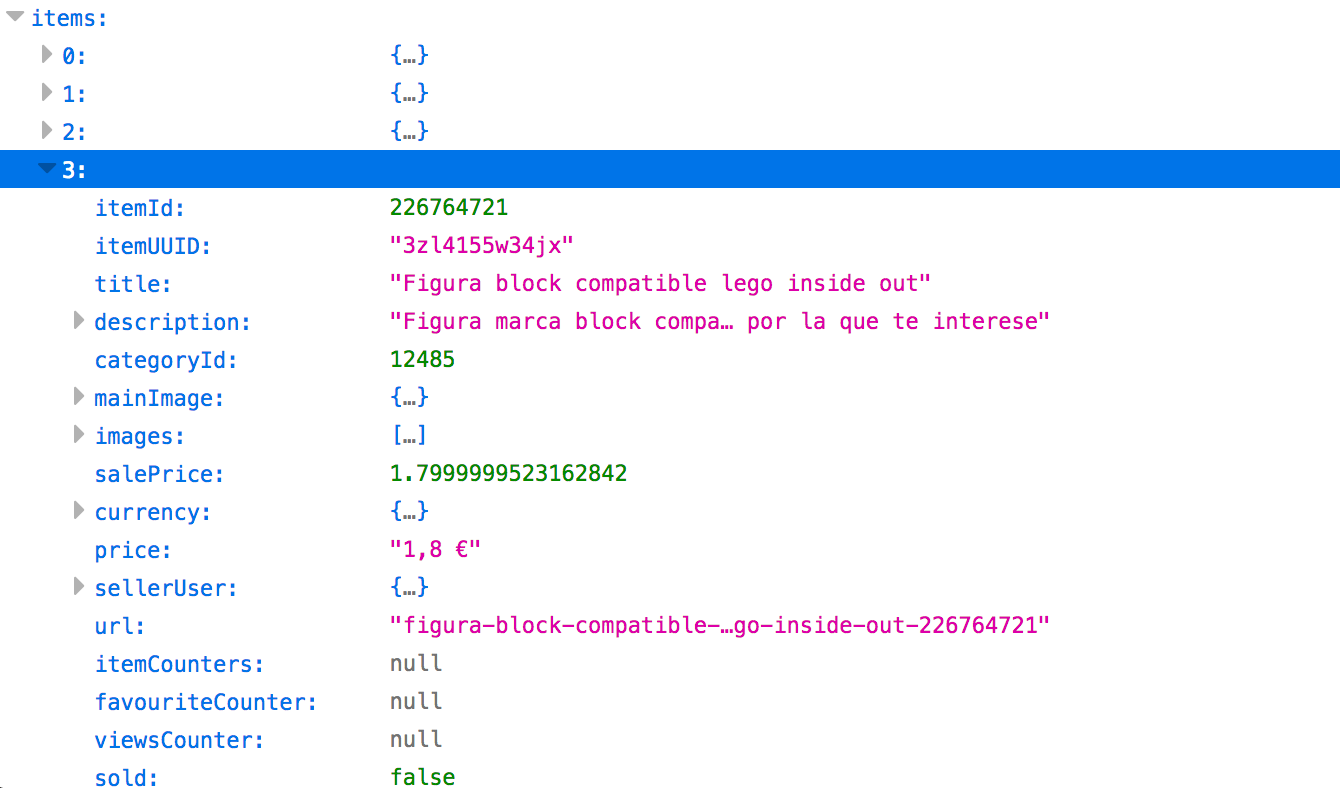
With a bit of luck, we’ll find what we want and we could build url requests as:
-
Get item:
Item ID: 226764721 http://pro2.wallapop.com/shnm-portlet/api/v1/item.json/{item_id} -
Get user:
User ID: 26329910 http://pro2.wallapop.com/shnm-portlet/api/v1/user.json/{user_id} -
Get sold items from user id:
Params: user_id=34592215; init=0; end=250 http://pro2.wallapop.com/shnm-portlet/api/v1/item.json/user2/{user_id}?init={}&end={end}&statuses=SOLD_OUTSIDE -
, etc.
APK problems
For each item or seller, Wallapop doesn’t always return the same parameters, so you should build (or use) a sort of ORM or key1-key2 mapping to fix these problems.
Crawler
Firsts of all, building a crawler looks easier than it really is. So I recommend either using one already built like Scrapy or be prepared for spending some time with weird errors.
To get sold items, we should:
- Get items from page 0 to n for each Spain province
- Get all the sellers from the previous scrape
- Get all sold items from the previously scrapped sellers.
Boosting its power
You can’t do the previous step using a sequential approach. For instance, if one request takes 2 seconds to send, receive and process it, with 5 million items it would take around 115 days to finish. Therefore, we need the power of parallelization, multithreading, async programming or whatever suit you best for this purpose.
Generally speaking, around 100-200 requests per second should be okay.
Limits
I have no idea what are real limits of Wallapop, but empirically I can say that right now, every IP doing more than 30req/s is going to get blocked for 10min.
Storing the data
Initially, I started using SQLite because it’s pretty convenient for storing and querying a dataset. But when I realized I had to use a connection pooling for storing the async request I had to migrate everything to MySQL.
Migrate this small dataset wasn’t hard, it wasn’t trivial either due to problems I’m not used to such as ASCII '\0', hex-blobs, collation problems, integers of 4 bytes, integers of 8 bytes, weird bugs in the SQLite dump process,… So okay, lesson learned.
Data description
- Items: 3,284,222
- Sellers: 221,290
- Item categories: 13
- Data size: ~1GB
- Others: Lots of outliers
Although this dataset is not incredibly massive, it’s big enough to force us to take a careful approach from an efficiency standpoint. (Even more, if we’re dealing with visualizations)
Data cleaning
Removing outliers
An outlier is an observation whose probability to occur is low. There are many methods which try to identify them and can be classified into parametric and non-parametric.
- Parametric methods: Assume some underlying distribution, such as Normal or LogNormal.
- Non-parametric methods: Don’t assume any distribution, such as Box plot or DBScan.
Additionally, we can perform a univariate analysis (one variable) or multivariate (more than one variable).
Most popular methods are usually the following:
- Common sense (a.k.a thresholds): “No chicken costs than 1M”
- Z-Score: Indicates how many standard deviations a data point is from the sample’s mean. (There is an enhanced more robust version)
- IRQ: Pretty robust, but depending on the case, it might be too conservative if the distribution is not normal.
- DBScan: Detect outliers in nonparametric distributions in many dimensions. (hard to tune).
- Isolation Forests: A bit of both (easy to optimize and robust).
Before we start with our data, we can make a few guesses:
- Distributions of prices for each category are expected to be non-parametric as each category contains many different products.
- We’ll have lots of outliers that will break the standard deviation and the mean, as many people set symbolic prices like ‘0€ or 1€’ for a car, house, etc. Or even billions of euros for an iPod.
- Prices tend to follow a lognormal distribution, so it should be a good candidate.
Anyway, let’s start with our data!
First, we need to know if we’re dealing with a parametric or non-parametric distribution.
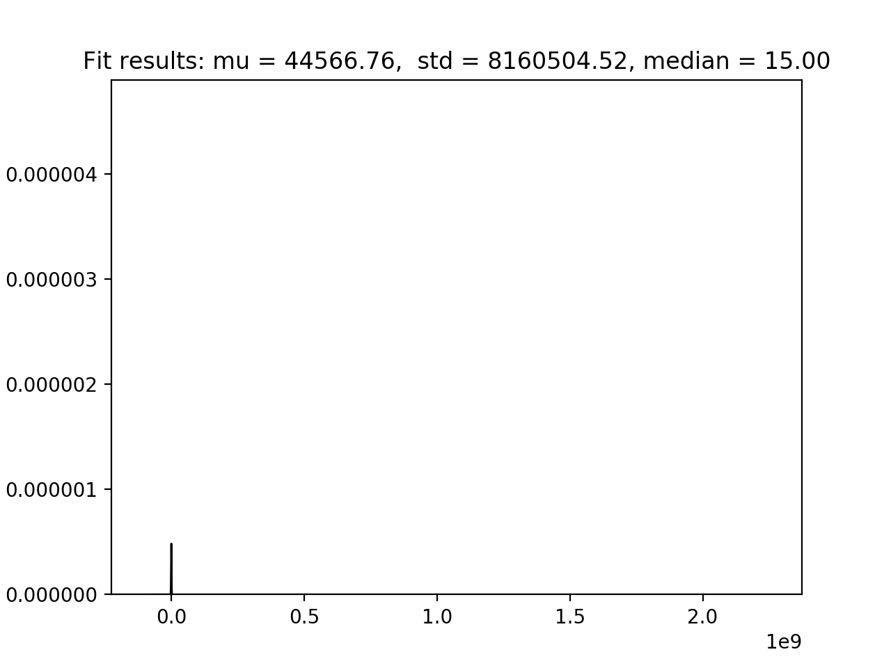
From the above image, we see nothing. However, we can guess that Z-Score is not going to be a good method to remove outliers as they’re pulling up the standard deviation.
After zooming in a bit the above image, we now see a strongly skewed non-parametric distribution heavily long-tailed. This means that removing outliers could get really tricky as there are so many of them strongly pulling up the standard deviation.

One option we have is to consider the distribution as parametric for the sake of simplicity and use a robust method to remove them, but in this case, it wouldn’t be a good idea as later we’ll see.
Outliers usually drop with multivariate analysis, so let’s compute stats based on each category to see if things get easier.
Coches                            sample_size=     40069;    q25=    1500.0;    q75=    6800.0;    iqr=    5300.0;    min_qval=   -6450.0;    max_qval=   14750.0;    min=         0;    max= 695479092;    median=    3000.0;    mean=     57723.72210;    std=     6010324.71305
Niños y Bebés                     sample_size=    314573;    q25=       5.0;    q75=      20.0;    iqr=      15.0;    min_qval=     -17.5;    max_qval=      42.5;    min=         0;    max= 619121873;    median=      10.0;    mean=     4801.87070;    std=     1448201.42496
Libros, Películas y Música        sample_size=    218423;    q25=       5.0;    q75=      20.0;    iqr=      15.0;    min_qval=     -17.5;    max_qval=      42.5;    min=         0;    max=2147483647;    median=      10.0;    mean=     14405.79696;    std=     4977604.40512
Moda y Accesorios                 sample_size=    850531;    q25=       5.0;    q75=      20.0;    iqr=      15.0;    min_qval=     -17.5;    max_qval=      42.5;    min=         0;    max=2147483647;    median=      10.0;    mean=     4872.58952;    std=     2595404.51731
Muebles, Deco y Jardín            sample_size=    397698;    q25=      10.0;    q75=      69.0;    iqr=      59.0;    min_qval=     -78.5;    max_qval=     157.5;    min=         0;    max= 999999999;    median=      25.0;    mean=     5601.92546;    std=     1906325.21787
Otros                             sample_size=    294379;    q25=       6.0;    q75=      45.0;    iqr=      39.0;    min_qval=     -52.5;    max_qval=     103.5;    min=         0;    max=1000000000;    median=      15.0;    mean=     28924.16016;    std=     4540633.42517
Electrónica                       sample_size=    404414;    q25=      15.0;    q75=     150.0;    iqr=     135.0;    min_qval=    -187.5;    max_qval=     352.5;    min=         0;    max=1000000000;    median=      50.0;    mean=     13785.01049;    std=     3399570.68320
Deporte y Ocio                    sample_size=    257783;    q25=      14.0;    q75=      80.0;    iqr=      66.0;    min_qval=     -85.0;    max_qval=     179.0;    min=         0;    max=2147483647;    median=      30.0;    mean=     13250.44203;    std=     4686248.59380
Motor y Accesorios                sample_size=    182464;    q25=      25.0;    q75=     250.0;    iqr=     225.0;    min_qval=    -312.5;    max_qval=     587.5;    min=         0;    max= 120000000;    median=      60.0;    mean=     2525.85975;    std=     435625.62062
Consolas y Videojuegos            sample_size=    145522;    q25=      10.0;    q75=      40.0;    iqr=      30.0;    min_qval=     -35.0;    max_qval=      85.0;    min=         0;    max=2147483647;    median=      20.0;    mean=     15745.92700;    std=     5635854.65372
Inmobiliaria                      sample_size=     14359;    q25=      20.0;    q75=     750.0;    iqr=     730.0;    min_qval=   -1075.0;    max_qval=    1845.0;    min=         0;    max= 169000000;    median=     100.0;    mean=     62468.05279;    std=     2227883.81974
Electrodomésticos                 sample_size=     79122;    q25=      15.0;    q75=     100.0;    iqr=      85.0;    min_qval=    -112.5;    max_qval=     227.5;    min=         0;    max=1000000000;    median=      39.0;    mean=     20356.53851;    std=     3666865.69689
Servicios                         sample_size=     25308;    q25=       3.0;    q75=      50.0;    iqr=      47.0;    min_qval=     -67.5;    max_qval=     120.5;    min=         0;    max=2147483647;    median=      15.0;    mean=     214405.77446;    std=     15817839.17886
Now we see some interesting things:
Min valuesandMax valuesare absolute nonsensemeanvalues are way too far from themedian(skewed distribution)standard deviationsare also way larger than they should.- Prices from “Inmobiliaria” (real state) are usually symbolic.
- All distributions are heavily long-tailed.
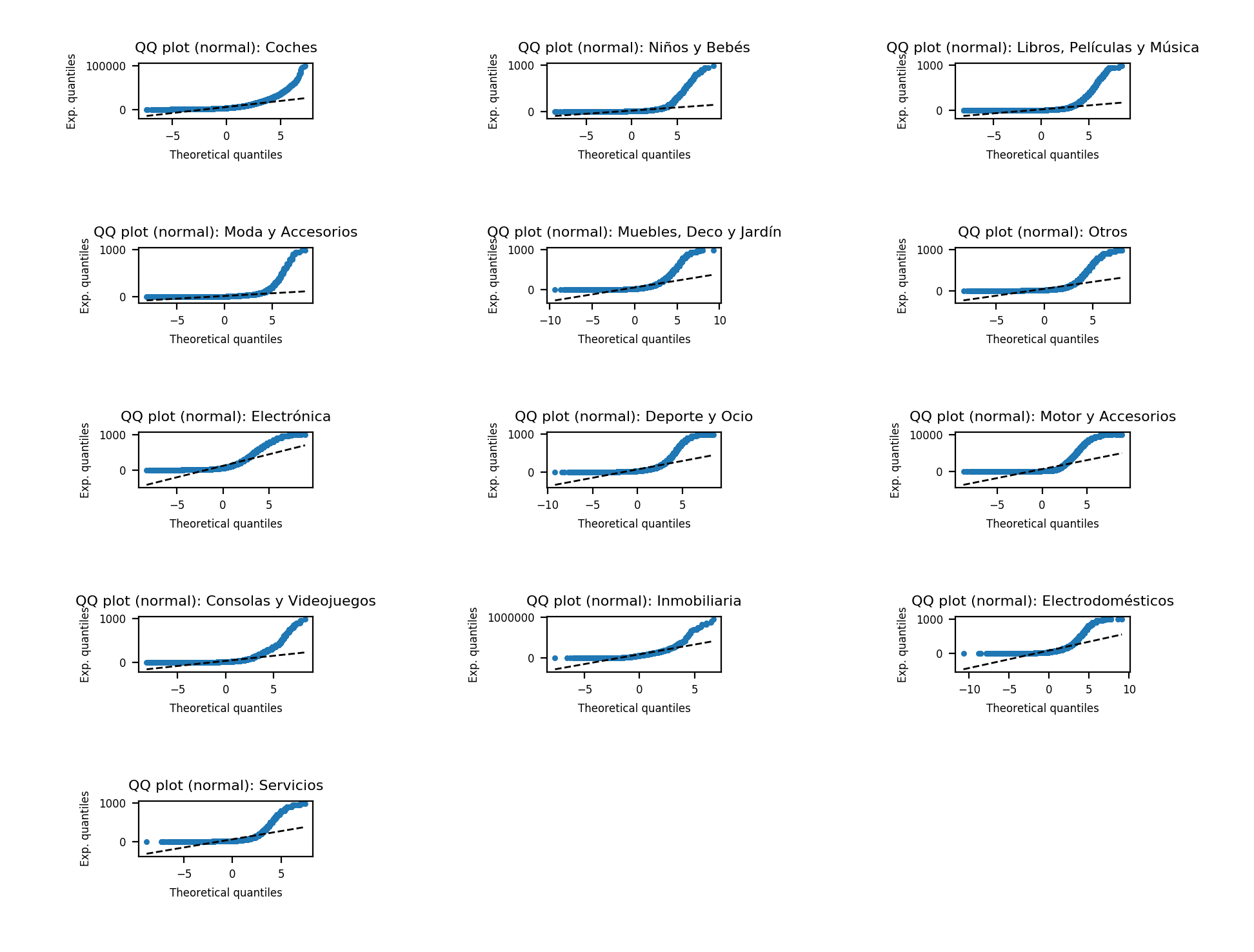
Our next step is to assess if our data how our data is distributed. To do this, we can use Q-Q plot (Quantile-Quantile plot). In this approach, quantiles of our data distribution are plotted against quantiles of a known distribution as a scatter plot. If distributions are similar the plot will be close to a straight line.
In the picture below, we test against a normal distribution. At first, it seems to be normal (ignoring some outliers), but then, after zoom in, we realize that outliers are too big and distort our view.
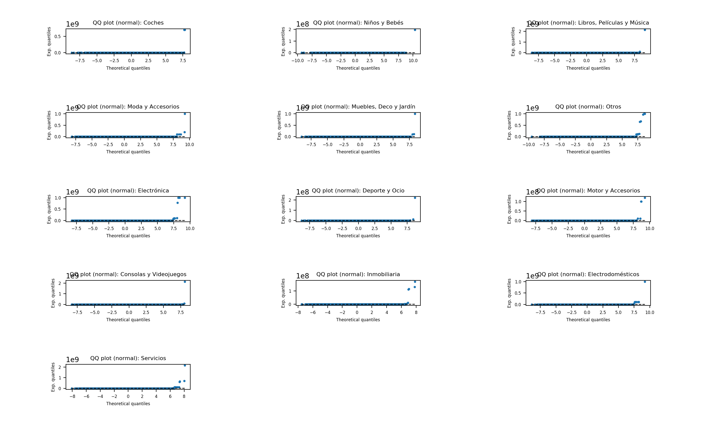
We shouldn’t assume that data our follow a normal distribution, at least not yet. First, we can try to remove some clearly strong outliers using a couple methods:
IQR: Good choice, but tuningPercentiles: too subjective without strong evidence to support our choices.Z-Score: is not robust enough due to the large standard deviations.Z-Score modified: better than above, but still not good enough*.Covariance estimators: similar to the above and requires a careful parameter tuning.One class SVM with a non-linear kernel (RBF): too slow.
Z-Score modifiedrefers to “Boris Iglewicz and David Hoaglin (1993), “Volume 16: How to Detect and Handle Outliers”, The ASQC Basic References in Quality Control: Statistical Techniques, Edward F. Mykytka, Ph.D., Editor.”
So far, the methods we’ve used to detect outliers didn’t work well. Hence, we can try a different (more subjective) approach. First, we create a histogram of the number of digits of each price for every category. And then, we can simply say “keep these columns” and consider the remaining columns as outliers (usually the ones with large slopes or small frequencies). (Note: This approach is almost the same as using a log10 function but more manual.)
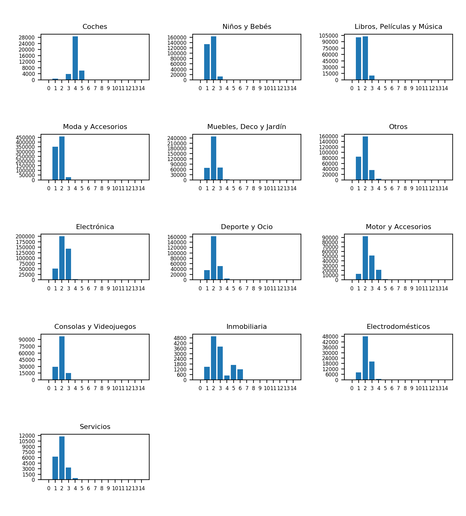
Interestingly, we notice that the “Inmobiliaria” (real state) plot has clearly two distributions overlapped. After taking a closer look, we realize that the 3rd and 4th split rental and purchase flats.
As we don’t have strong outliers anymore, we can try to make Q-Q plot again. Now, all distributions have become clearly not normal. Indeed, this was expected because each category contains many products and every product have different distribution (probably normal).
Refining outliers detection
Now the category summary stats look better but at the same time, it seems like the cutting points are too arbitrary (e.g.: 9999 -> yes, but 10,000 no).
Coches                            sample_size=     38216;    q25=    1657.0;    q75=    6999.0;    iqr=    5342.0;    min_qval=   -6356.0;    max_qval=   15012.0;    min=        99;    max=     99900;    median=    3300.0;    mean=     5639.45625;    std=     6714.73688
Niños y Bebés                     sample_size=    301542;    q25=       5.0;    q75=      20.0;    iqr=      15.0;    min_qval=     -17.5;    max_qval=      42.5;    min=         2;    max=       990;    median=      10.0;    mean=     24.74558;    std=     54.70934
Libros, Películas y Música        sample_size=    205980;    q25=       5.0;    q75=      20.0;    iqr=      15.0;    min_qval=     -17.5;    max_qval=      42.5;    min=         2;    max=       995;    median=      10.0;    mean=     25.41273;    std=     61.22507
Moda y Accesorios                 sample_size=    820862;    q25=       5.0;    q75=      20.0;    iqr=      15.0;    min_qval=     -17.5;    max_qval=      42.5;    min=         2;    max=       998;    median=      10.0;    mean=     22.92911;    std=     48.67112
Muebles, Deco y Jardín            sample_size=    382046;    q25=      12.0;    q75=      70.0;    iqr=      58.0;    min_qval=     -75.0;    max_qval=     157.0;    min=         2;    max=      9969;    median=      30.0;    mean=     78.09835;    std=     217.16205
Otros                             sample_size=    271115;    q25=       8.0;    q75=      50.0;    iqr=      42.0;    min_qval=     -55.0;    max_qval=     113.0;    min=         2;    max=      9990;    median=      20.0;    mean=     98.97225;    std=     438.21540
Electrónica                       sample_size=    388968;    q25=      18.0;    q75=     160.0;    iqr=     142.0;    min_qval=    -195.0;    max_qval=     373.0;    min=         2;    max=      9900;    median=      55.0;    mean=     136.59570;    std=     235.89987
Deporte y Ocio                    sample_size=    247761;    q25=      15.0;    q75=      85.0;    iqr=      70.0;    min_qval=     -90.0;    max_qval=     190.0;    min=         2;    max=      9800;    median=      35.0;    mean=     114.70733;    std=     345.04093
Motor y Accesorios                sample_size=    172649;    q25=      30.0;    q75=     258.0;    iqr=     228.0;    min_qval=    -312.0;    max_qval=     600.0;    min=         2;    max=     96000;    median=      70.0;    mean=     659.71477;    std=     2220.59380
Consolas y Videojuegos            sample_size=    138106;    q25=      10.0;    q75=      40.0;    iqr=      30.0;    min_qval=     -35.0;    max_qval=      85.0;    min=         2;    max=       990;    median=      20.0;    mean=     42.25236;    std=     65.81536
Inmobiliaria                      sample_size=     13162;    q25=      30.0;    q75=    1400.0;    iqr=    1370.0;    min_qval=   -2025.0;    max_qval=    3455.0;    min=         2;    max=    950000;    median=     125.0;    mean=     24895.65317;    std=     70712.77978
Electrodomésticos                 sample_size=     76066;    q25=      15.0;    q75=     100.0;    iqr=      85.0;    min_qval=    -112.5;    max_qval=     227.5;    min=         2;    max=      9886;    median=      40.0;    mean=     107.14339;    std=     260.27639
Servicios                         sample_size=     19478;    q25=      10.0;    q75=      65.0;    iqr=      55.0;    min_qval=     -72.5;    max_qval=     147.5;    min=         2;    max=      9500;    median=      20.0;    mean=     128.37899;    std=     497.91525
So what can we do to smooth these cuts? Simple, find subcategories (here, products) in the main category and then find outliers as we normally do.
If we don’t want to find subcategories, we could try to compute the stats using our dataset and use them to remove outliers in the dirty dataset. As an example, if the most expensive item in the electronic categories cost 998€, we can now set the maximum to Q75 + (IQR * 1.5) which for this case is 352.5€ (too low).
Also, we could see how prices fit in different theoretical distributions such as LogNorm and remove outliers using that function as ideal distribution (see Gibrat’s law). Furthermore, it comes to my mind that we could compute the Gaussian KDE distribution (for example) using the “cleaner” data and then remove outliers using the Z-score method.
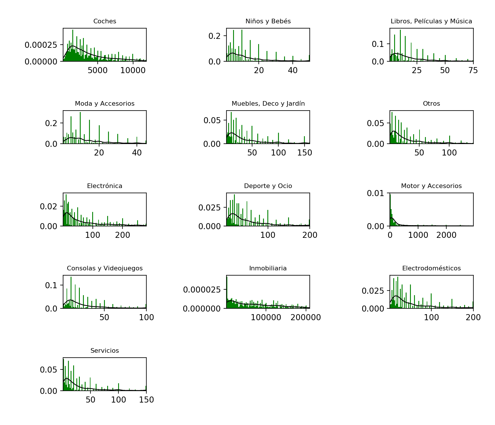
Note: I plotted up to the 90 percentile
As expected, it didn’t work well. As far as I know, I think only finding subcategories would work relatively well because many prices tend to concentrate around specific “pretty” values which should vary depending on the products.
On the other hand, we can try to refine just one type of outliers: “Prices for which sale price is 1€”. Sometimes it’s symbolic, sometimes is not. So what can we do about it from a general view? Plot them!
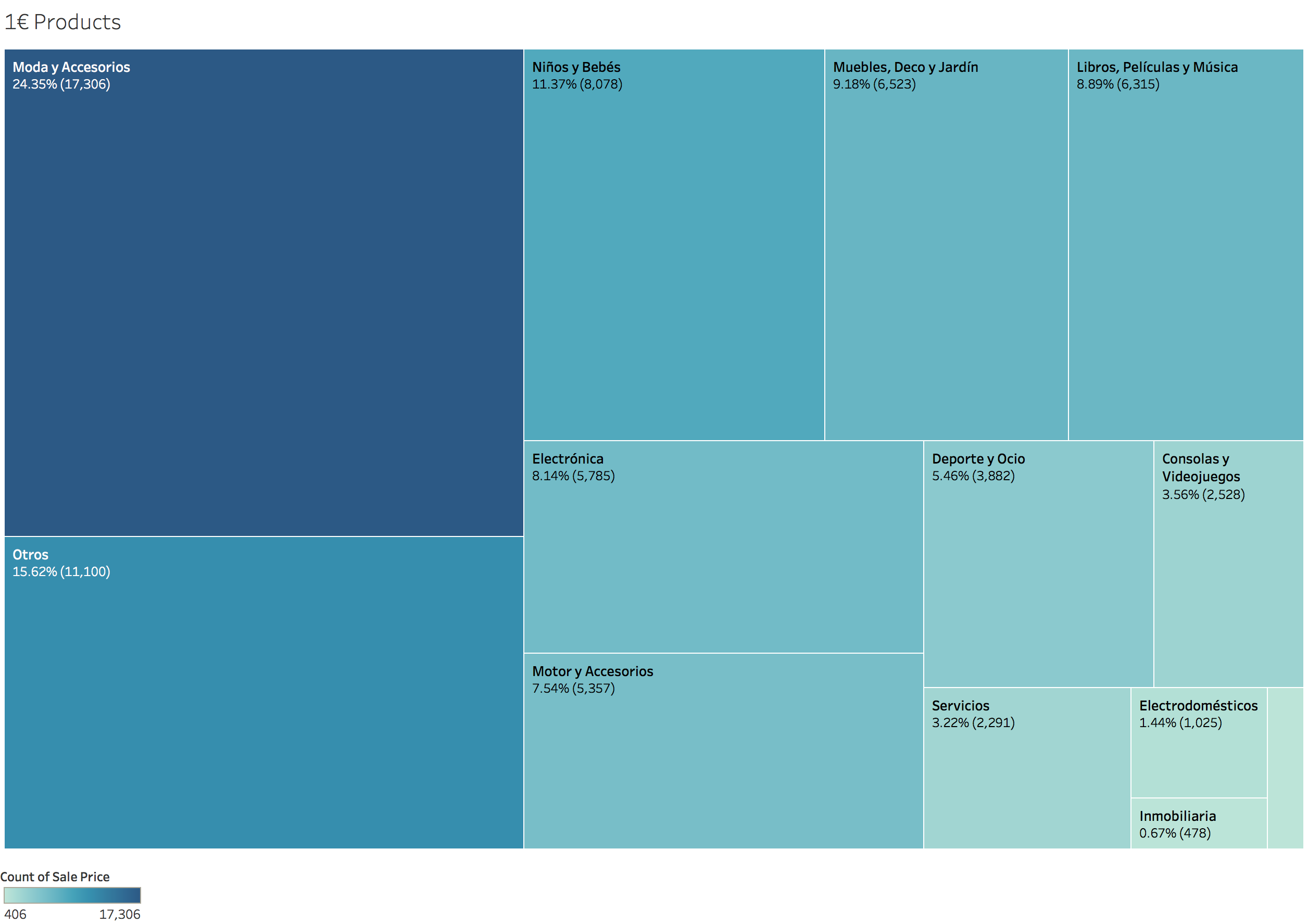
Now we see that although 1€ prices can be symbolic, in categories as “Moda” (Fashion) are more common than in “Coches” (cars). This means that taking into account the total number of items, most people don’t use 1€ to set a price as symbolic. We can infer that approximately between 1 to 3% of this prices are symbolic guessing from the “Coches” and “Inmobiliaria” categories.
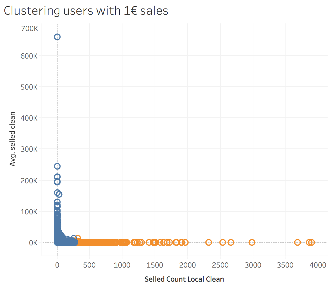
Moreover, we can plot the number of sales against the average earnings per user. Then, using a clustering model such as K-means we can cluster users into “casual users” and “pro users”. “Pro users” with many sales and low averages will probably sell real 1€ products.
And for the end, the most obvious refining. Find keywords in the description of 1€ products that lead us to think that a specific item has a symbolic price [e.g.: “Precio negotiable”]
There ares still many outliers, but we want them. The ones we didn’t want were the non-sense values. Hence, the final stats:
Coches                            sample_size=     38216;    q25=    1657.0;    q75=    6999.0;    iqr=    5342.0;    min_qval=   -6356.0;    max_qval=   15012.0;    min=        99;    max=     99900;    median=    3300.0;    mean=     5639.45625;    std=     6714.73688
Niños y Bebés                     sample_size=    309490;    q25=       5.0;    q75=      20.0;    iqr=      15.0;    min_qval=     -17.5;    max_qval=      42.5;    min=         1;    max=       990;    median=      10.0;    mean=     24.13577;    std=     54.13275
Libros, Películas y Música        sample_size=    211875;    q25=       5.0;    q75=      20.0;    iqr=      15.0;    min_qval=     -17.5;    max_qval=      42.5;    min=         1;    max=       995;    median=      10.0;    mean=     24.73350;    std=     60.50070
Moda y Accesorios                 sample_size=    837749;    q25=       5.0;    q75=      20.0;    iqr=      15.0;    min_qval=     -17.5;    max_qval=      42.5;    min=         1;    max=       998;    median=      10.0;    mean=     22.48707;    std=     48.27655
Muebles, Deco y Jardín            sample_size=    387966;    q25=      10.0;    q75=      70.0;    iqr=      60.0;    min_qval=     -80.0;    max_qval=     160.0;    min=         1;    max=      9969;    median=      27.0;    mean=     76.92190;    std=     215.70598
Otros                             sample_size=    281390;    q25=       7.0;    q75=      50.0;    iqr=      43.0;    min_qval=     -57.5;    max_qval=     114.5;    min=         1;    max=      9990;    median=      17.0;    mean=     95.39478;    std=     430.53260
Electrónica                       sample_size=    393858;    q25=      15.0;    q75=     160.0;    iqr=     145.0;    min_qval=    -202.5;    max_qval=     377.5;    min=         1;    max=      9900;    median=      50.0;    mean=     134.91219;    std=     234.91121
Deporte y Ocio                    sample_size=    251104;    q25=      15.0;    q75=      80.0;    iqr=      65.0;    min_qval=     -82.5;    max_qval=     177.5;    min=         1;    max=      9800;    median=      30.0;    mean=     113.19352;    std=     342.98411
Motor y Accesorios                sample_size=    177617;    q25=      30.0;    q75=     250.0;    iqr=     220.0;    min_qval=    -300.0;    max_qval=     580.0;    min=         1;    max=     96000;    median=      65.0;    mean=     641.29032;    std=     2192.01078
Consolas y Videojuegos            sample_size=    140179;    q25=      10.0;    q75=      40.0;    iqr=      30.0;    min_qval=     -35.0;    max_qval=      85.0;    min=         1;    max=       990;    median=      20.0;    mean=     41.64231;    std=     65.51639
Inmobiliaria                      sample_size=     13162;    q25=      30.0;    q75=    1400.0;    iqr=    1370.0;    min_qval=   -2025.0;    max_qval=    3455.0;    min=         2;    max=    950000;    median=     125.0;    mean=     24895.65317;    std=     70712.77978
Electrodomésticos                 sample_size=     76066;    q25=      15.0;    q75=     100.0;    iqr=      85.0;    min_qval=    -112.5;    max_qval=     227.5;    min=         2;    max=      9886;    median=      40.0;    mean=     107.14339;    std=     260.27639
Servicios                         sample_size=     19478;    q25=      10.0;    q75=      65.0;    iqr=      55.0;    min_qval=     -72.5;    max_qval=     147.5;    min=         2;    max=      9500;    median=      20.0;    mean=     128.37899;    std=     497.91525
Exploratory Data Analysis
“EDA is an attitude”. This means that we have to find the main characteristics of our dataset rather than following a specific set of techniques.
Notes on
R-Squared: It’s a statistical measure of how close the data are to the fitted regression line. In other words, how well our model explains the response data. Range from 0 to 100%, the higher usually the better. But a high value should be double check using a residual plot or similar. Also a low value could be intrinsic to the variability of the data we’re trying to model.
Descriptive statistics
Mmmh… Bla, bla, bla
Data visualization
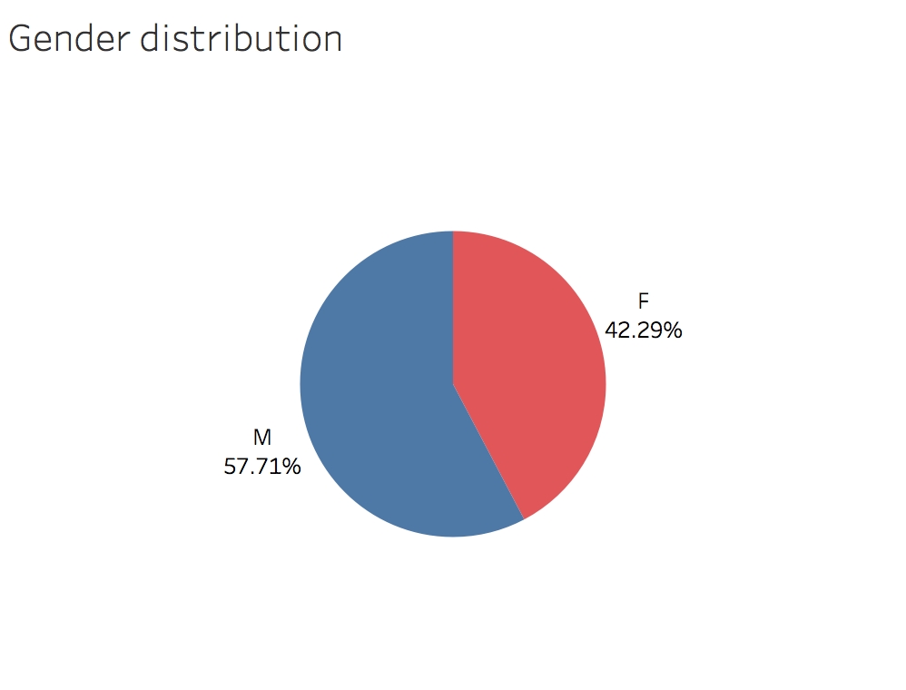
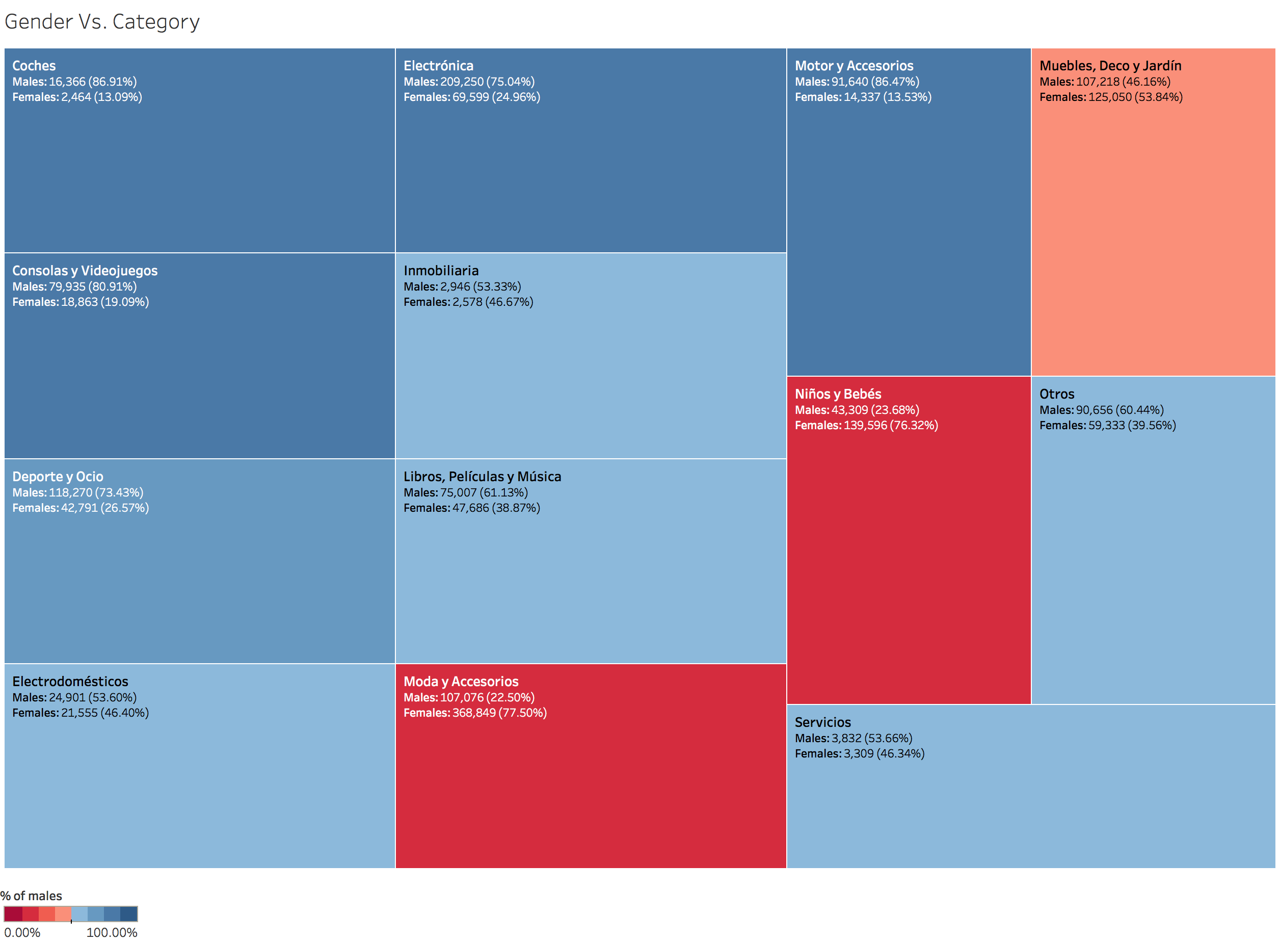
Sellers
This app is slightly more popular amongst men than women. Although it’s interesting to notice some categories are more popular depending on the gender.
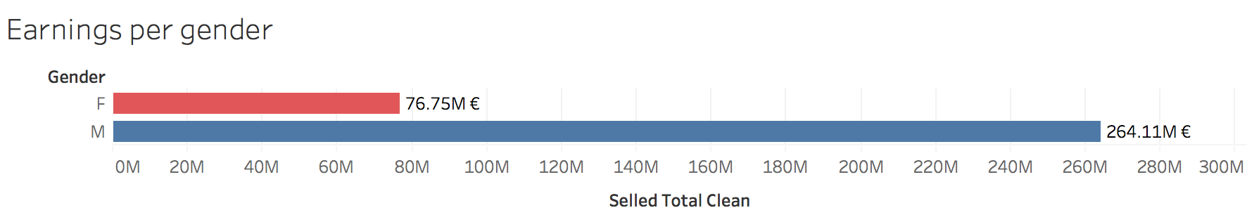
Total earnings per gender:
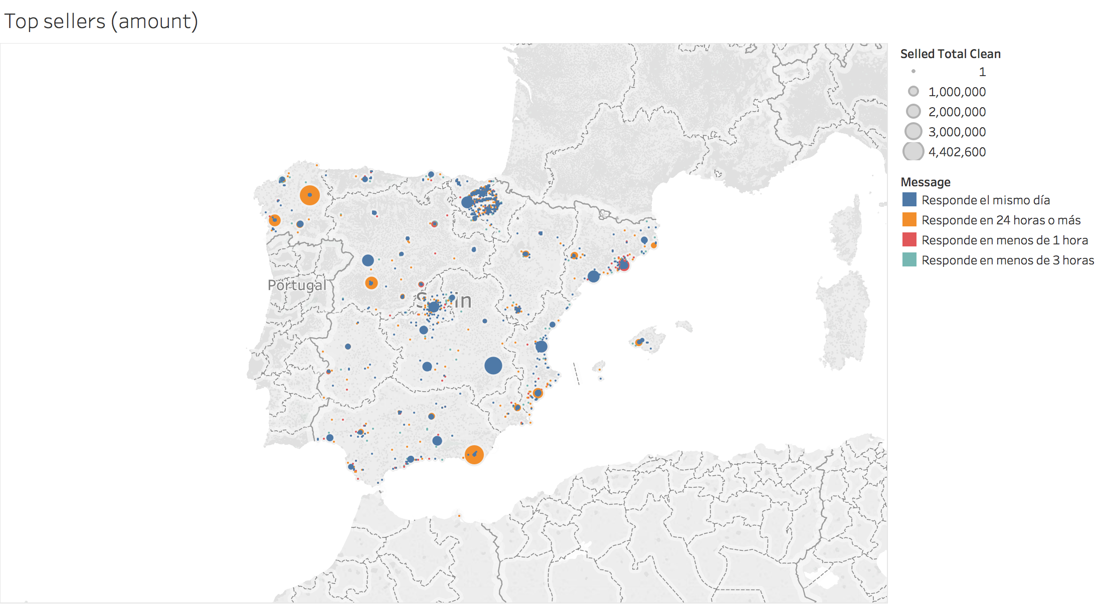
Geographical distributions
Total earnings per seller in Spain:
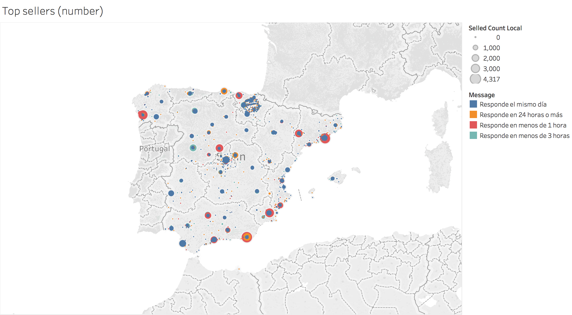
Number of sales per seller in Spain:
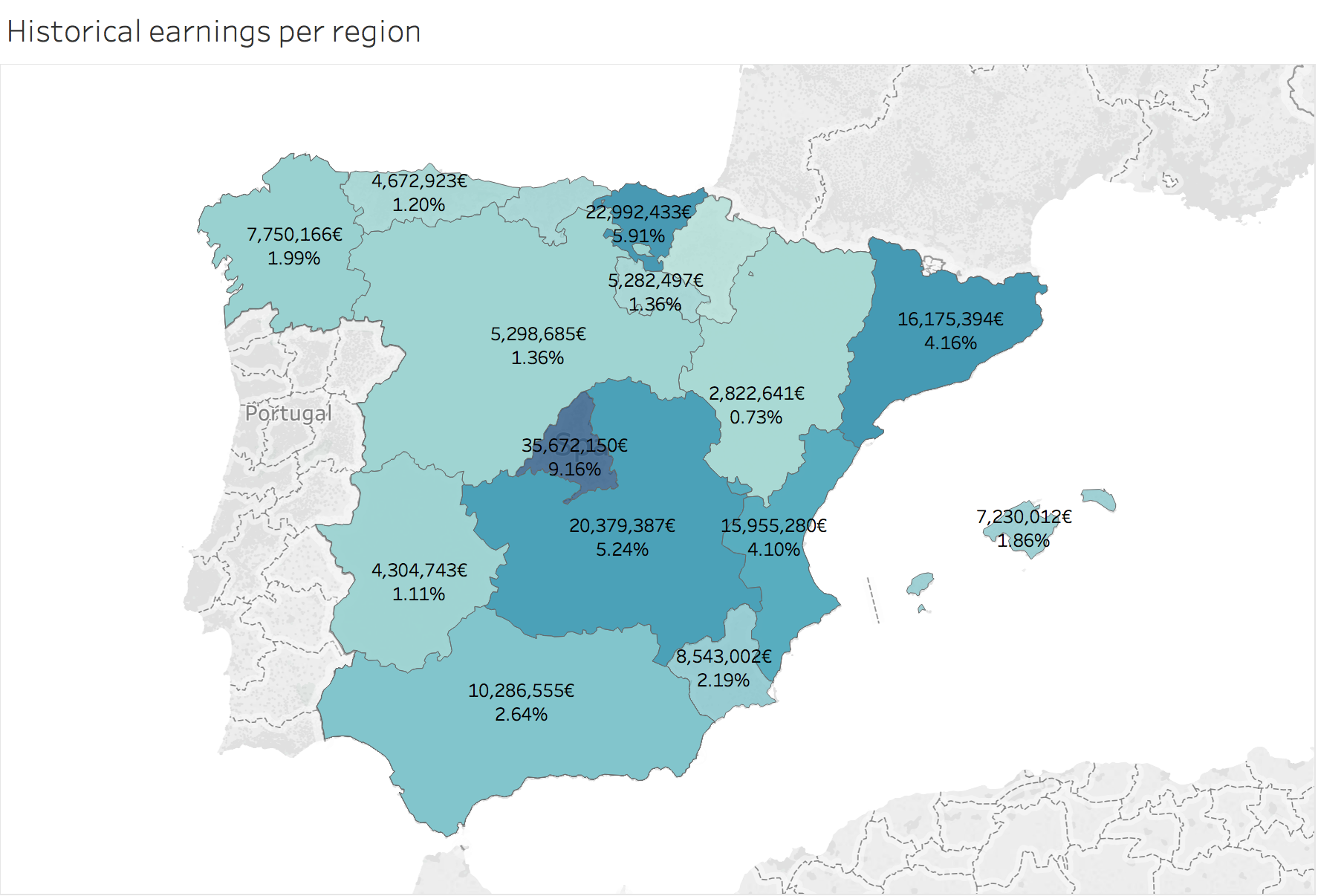
Historical earnings per region: (From -September 14, 2013- to -May 17, 2018)
This means that during 4 years and 8 months, the lower bound for the total amount of transactions in Spain is 389,275,717€ (the least). Most of these transactions are completely hidden from the tax agencies.
Custering sellers
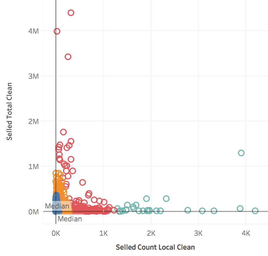
Relation between earnings and sales:
One can use a scatter plot to see the relation between total earnings and total sales. Next, we can fit a trend line (here, it had an R-squaredand P-value to low is not significant) and also, find clusters of users. In the picture below we discover that sellers with many sales are usually people and sellers with high earnings tend to be companies.
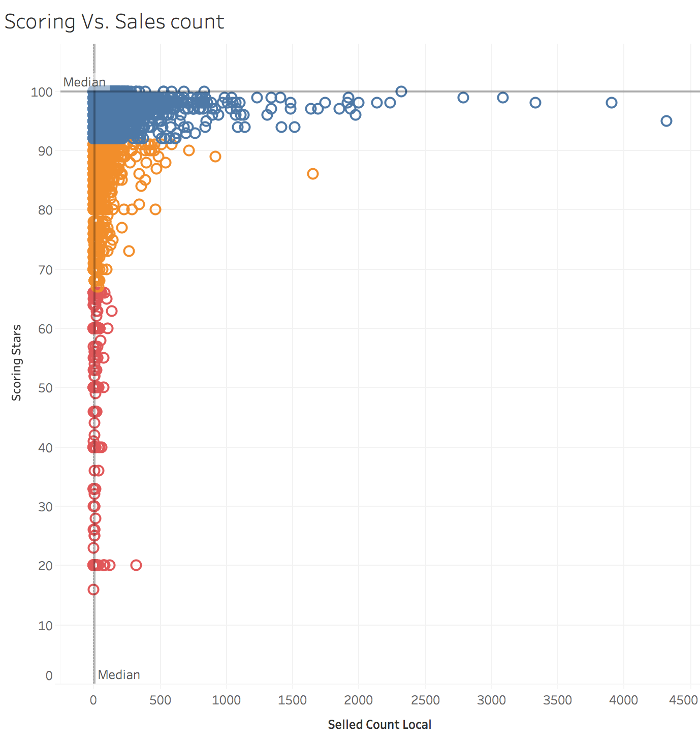
Relation between Scorings and number of sales:
Here, plain and simple: “If you sell bad quality products, you won’t last”. (Different colors cluster sellers into: good, normal and bad)
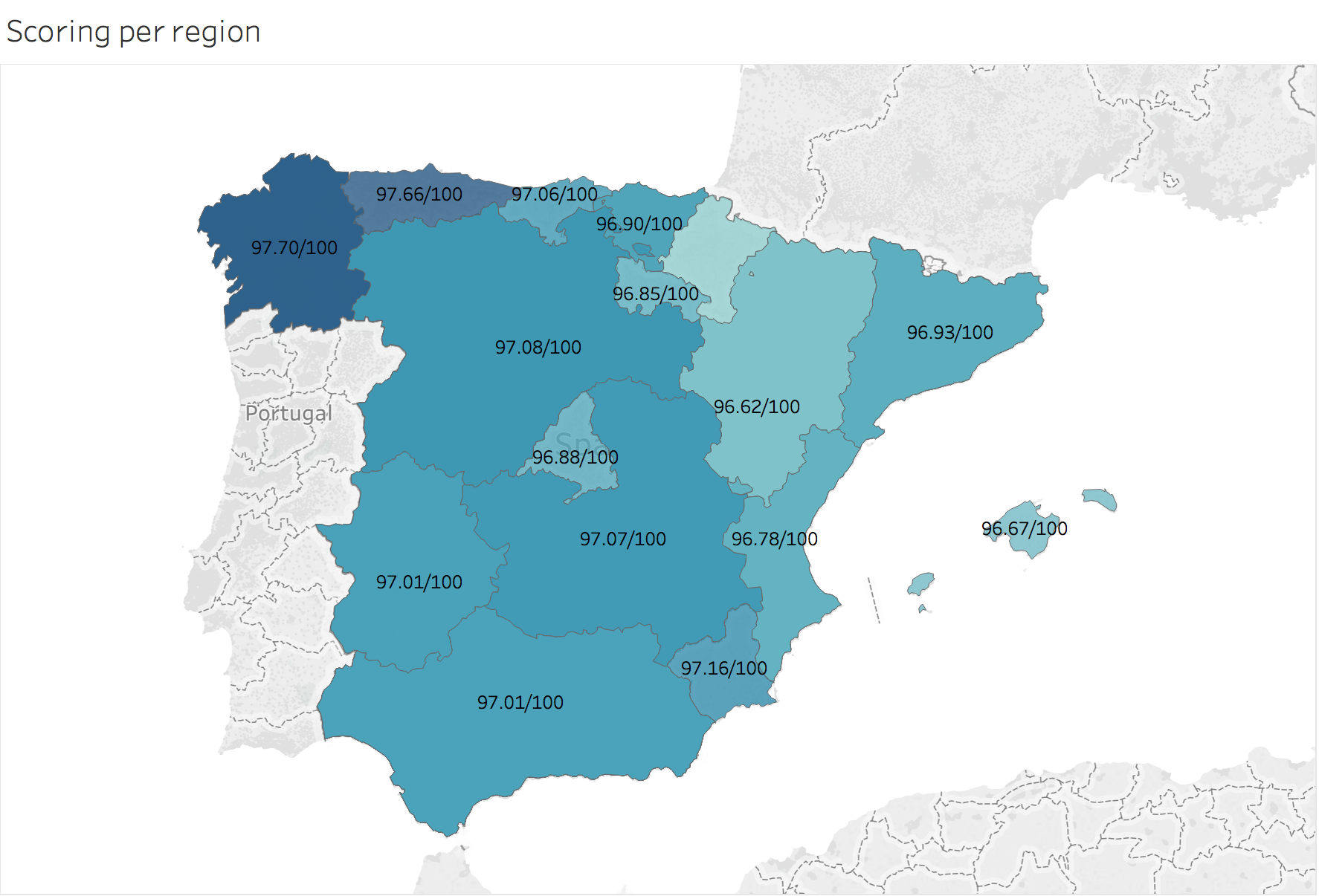
Scoring per region:
Scoring is averaged per region, and they seem to be pretty similar in all Spain.
Prices
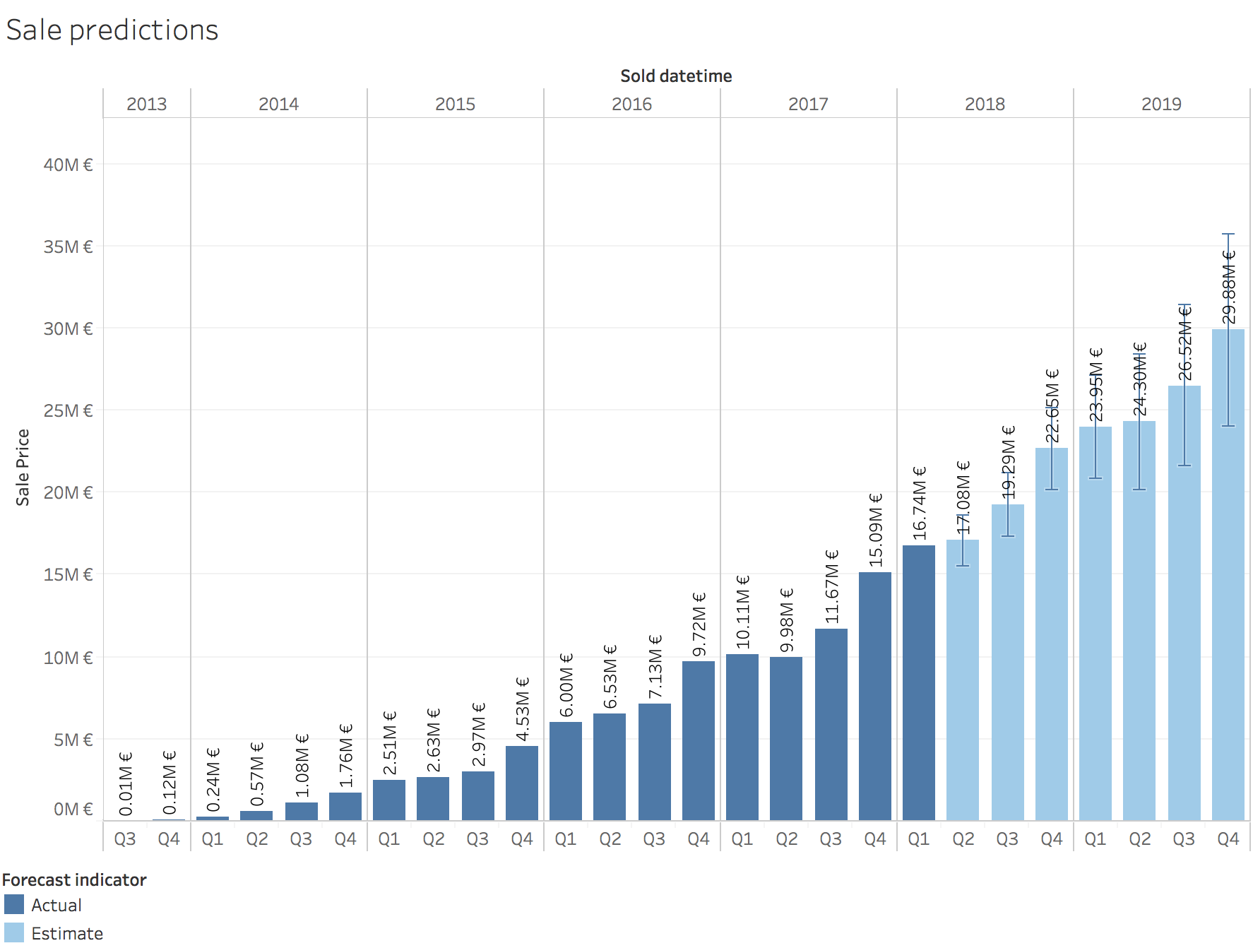
Sale predictions:
Sales evolution per category:
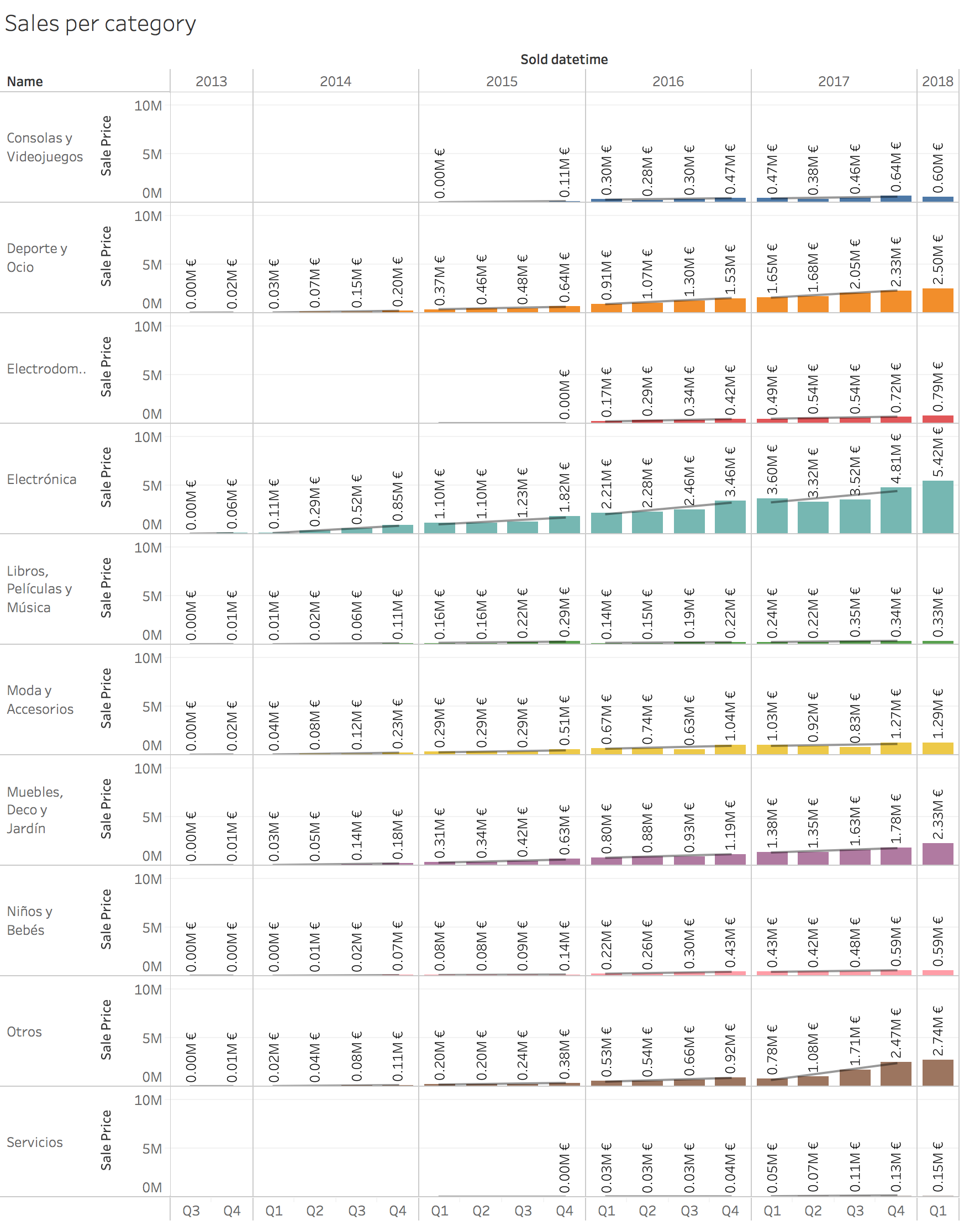
Disclaimer: “Inmobiliaria”, “Coches” and “Motor y accesorios” were excluded in order to ease the visualization.
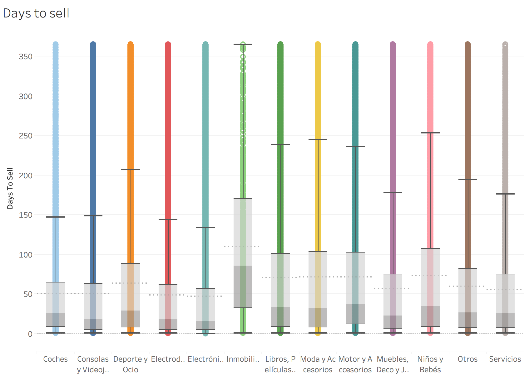
Days to sell:
I’ve just plotted items which took between 0 to 365 days to be sold. The average item is sold in 88 days (median in 30) and the product that took longer to sell, was a raincoat for the price of 5€ in the correct category (Moda y Accesorios), which did it in 4 Years, 3 Months and 3 Weeks (1573 days).
After digging a bit into those extreme cases, I discover that many people install the app and then, they forget about it.
Days to sell (Heatmap)
Color references Days to sell and size Number of sales.
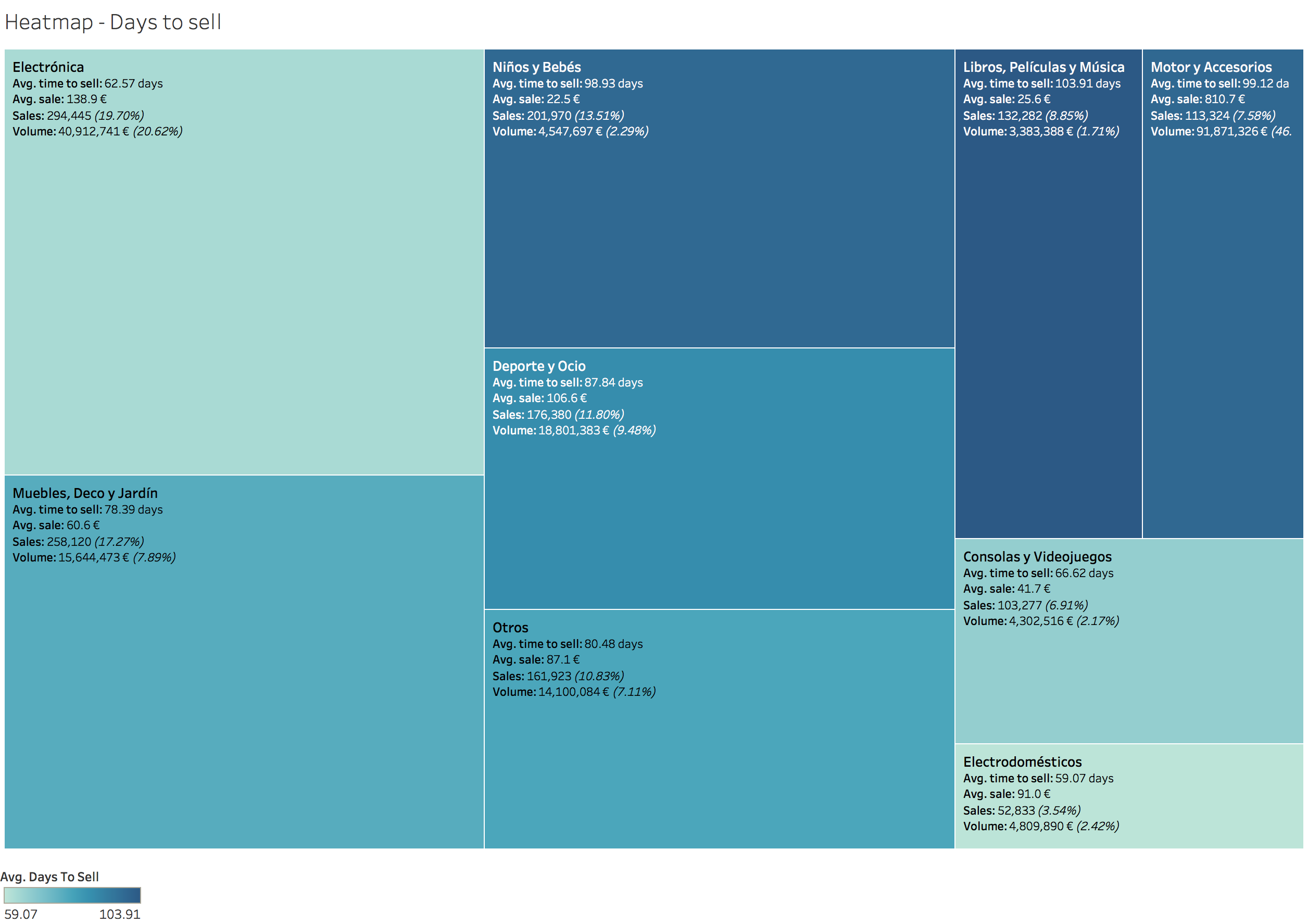
Disclaimer: “Inmobiliaria”, “Coches”, “Motor y Accesorios” and “Servicios” categories have been excluded.
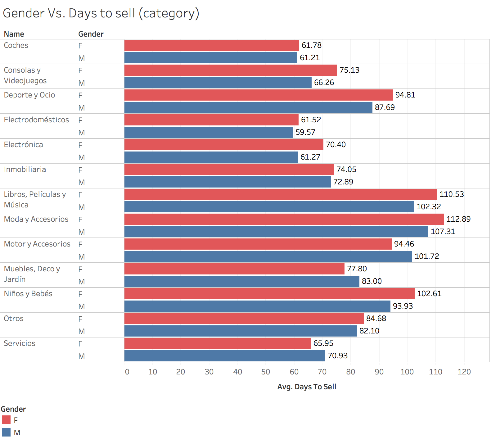
Days to sell (Gender)
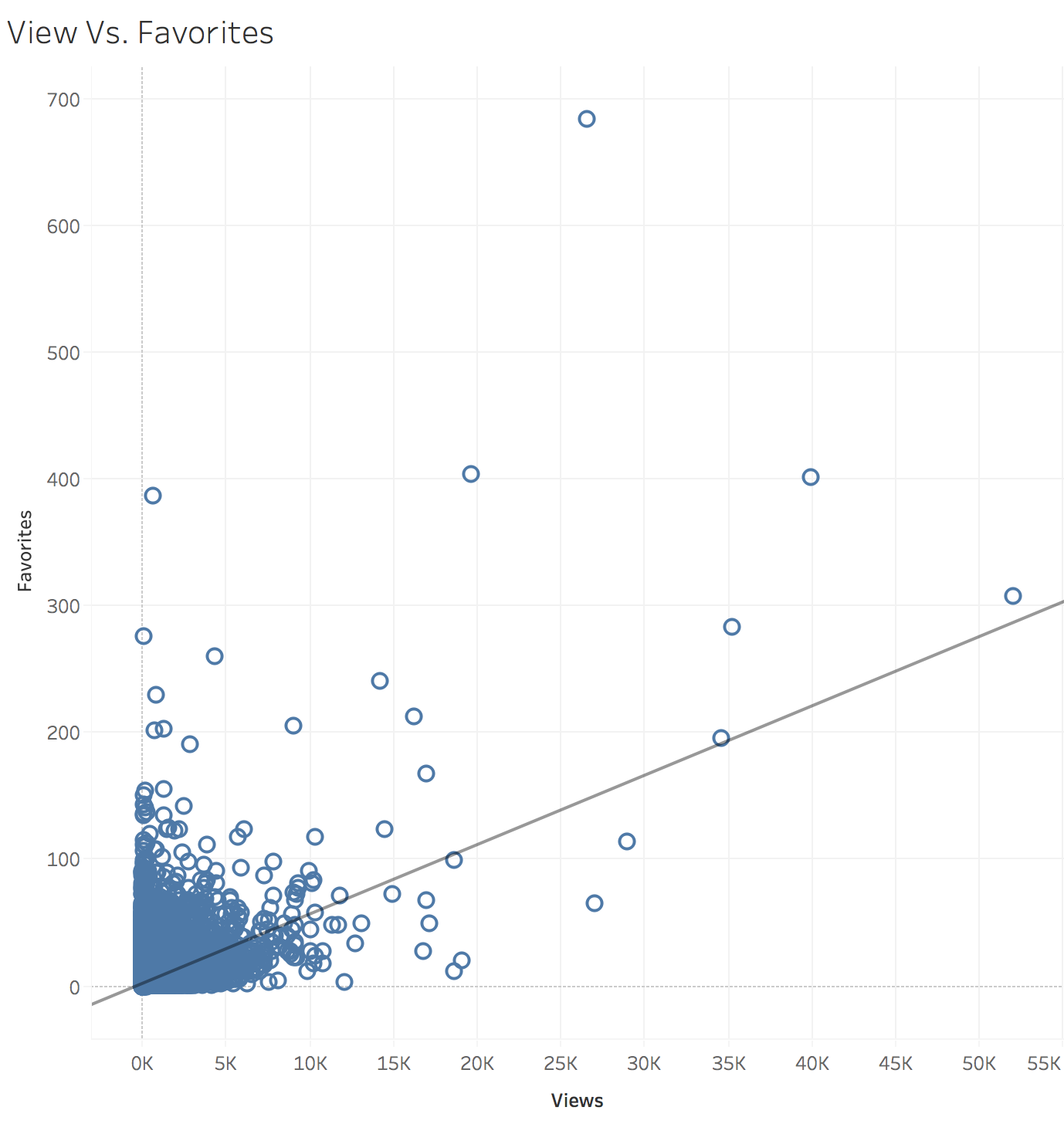
Views Vs. Favorites:
R-Squared is 0.1557. Need a review! I don’t understand this plot.
Note:
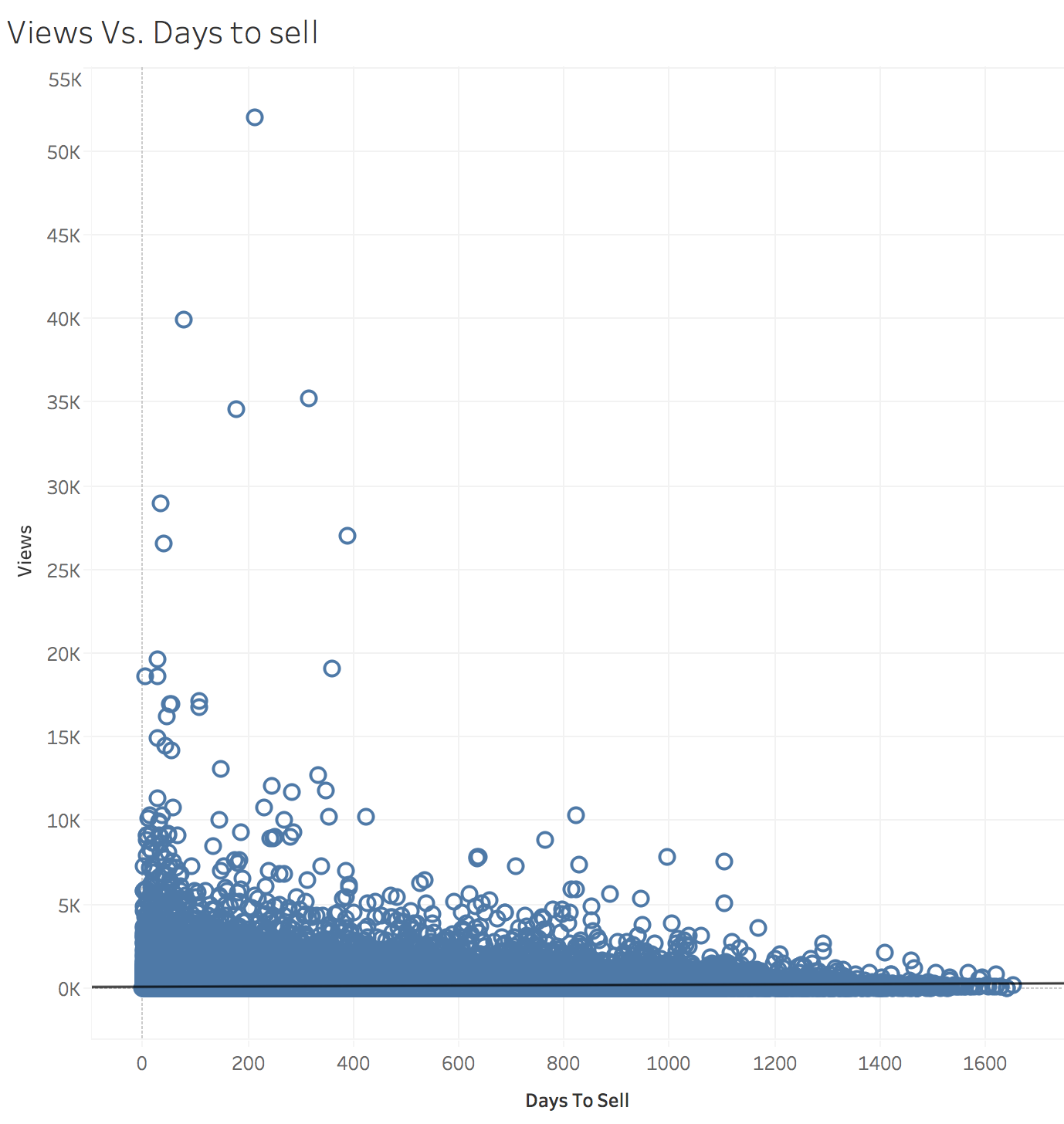
R-Squaredexplains Views Vs. Days to sell:
R-Squared is 0.0087. Need a review! I don’t understand this plot.
Sale price Vs. Original price:
R-Squared is 0.9888. We can infer that sellers are not fans of discounts, a relation which we will study after this paragraph.
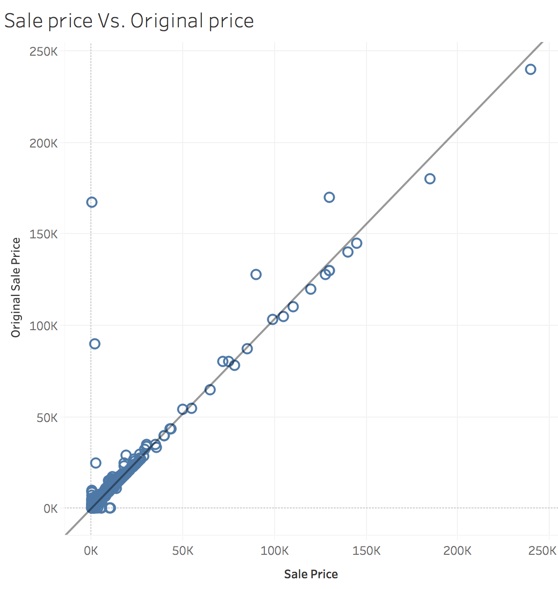
Disclaimer: Sample of 100,000 prices. All prices located on the axes were removed (user errors).
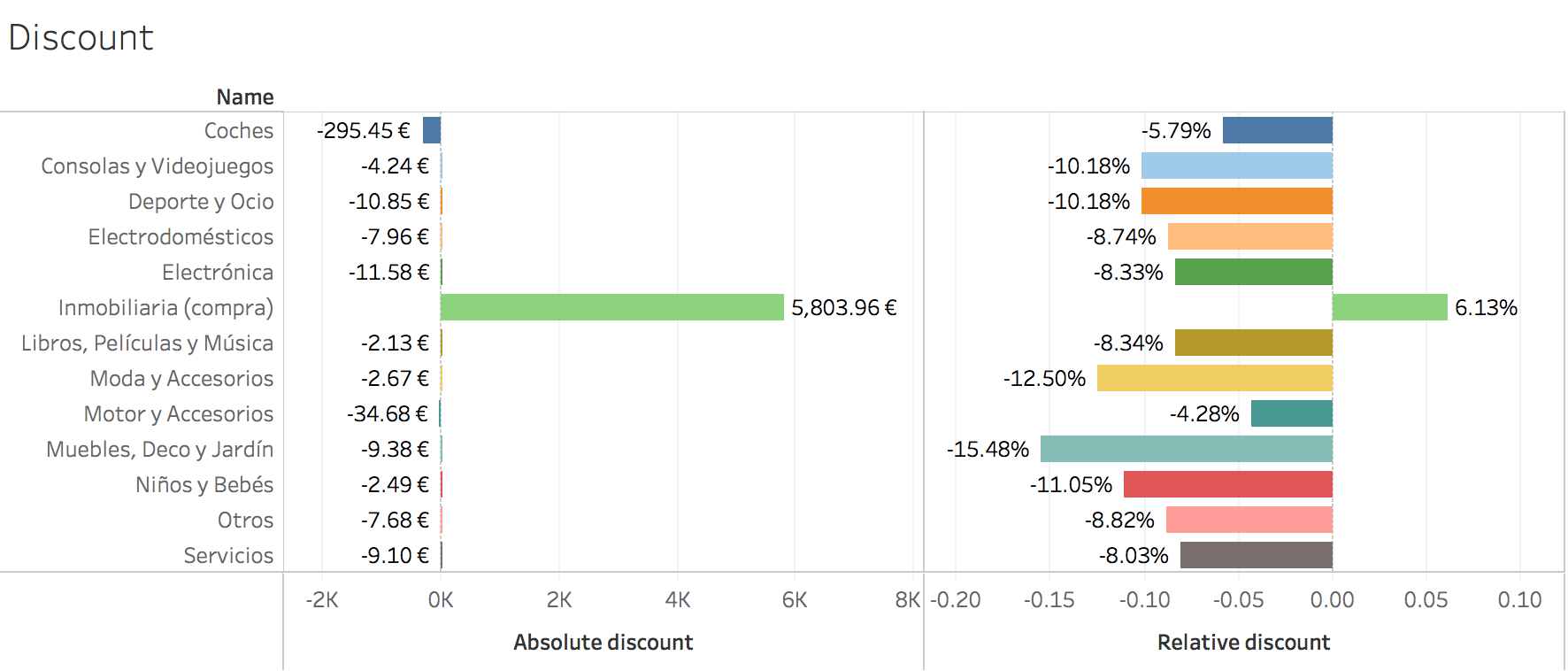
Discounts:
As there are many products in each category we should take these values with a grain of salt. But generally speaking, people usually decrease the price of a product when they want to sell it faster. It’s important to point out that I’ve removed all products I could from “Inmobiliaria” that are not a purchase (mainly rentals).
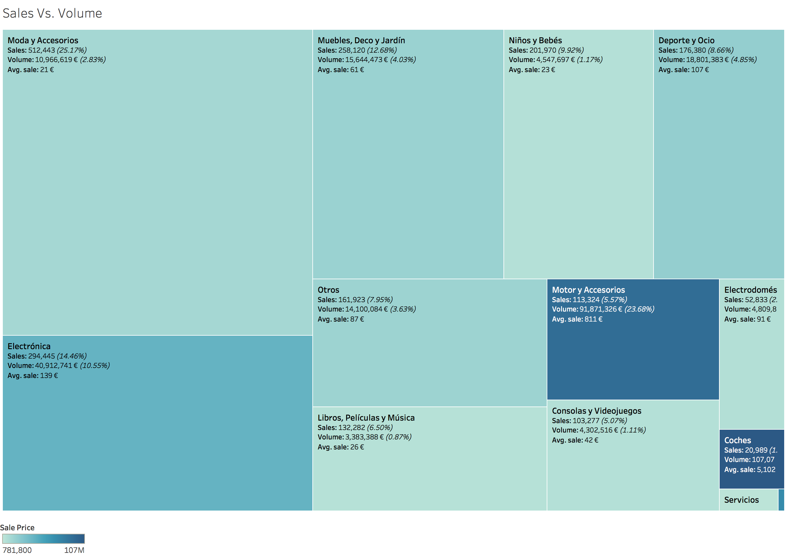
Sale counts Vs. Volume:
Color references Volume of sales and size Number of sales.